Redox oscillation

The set of ODEs for this system is [DOS2019]:

\[\begin{split}\frac{dD_{1}}{dt} &= p - aA D_{1} -d D_{1}\\ \frac{dD_{2}}{dt} &= dD_{1} - eD_{2}\\ \frac{dR}{dt} &= eD_{2} - qR\\ \frac{dA}{dt} &= bIR - aAD_{1}\end{split}\]

and the stability matrix:

\[\begin{split}\begin{equation} \mathbb{A}(\mathbf{x}(t), t) = \begin{pmatrix} -d -aA & 0 & 0 & -aD_{1}\\ d & -e & 0 & 0\\ 0 & e & -q & 0\\ -aA & 0 & b(1-a) & -bR -aD_{1} \end{pmatrix} \end{equation}\end{split}\]

1. Generate the input file containing the ODE system and the hard code the stability matrix, inside multiflap/odes/redox_oscillation.py:

   class RedoxModel:
       def __init__(self, a=1000, b=2, c=10000, d=0.2, e=0.1, q=0.1, p=1):
   
           self.a = a
           self.b = b
           self.c = c
           self.d = d
           self.e = e
           self.q = q
           self.p = p
           self.dimension = 4
       def dynamics(self, x0, t):
   
           """ODE system
           This function will be passed to the numerical integrator
   
           Inputs:
               x0: initial values
               t: time
   
           Outputs:
               x_dot: velocity vector
           """
           D1, D2, R, A = x0
           dD1_dt = self.p - self.a*A*D1 - self.d*D1
           dD2_dt = self.d*D1 - self.e*D2
           dR_dt = self.e*D2 - self.q*R
           dA_dt = self.b*(1-A)*R - self.a*A*D1
   
           vel_array = np.array([dD1_dt, dD2_dt, dR_dt, dA_dt], float)
           return vel_array
   
   
   
       def get_stability_matrix(self, x0, t):
   
           """
           Stability matrix of the ODE system
   
           Inputs:
               x0: initial condition
           Outputs:
               A: Stability matrix evaluated at x0. (dxd) dimension
               A[i, j] = dv[i]/dx[j]
           """
           D1, D2, R, A = x0
           A_matrix = np.array([[-self.d - self.a*A,  0., 0.,-self.a*D1],
                         [self.d,  -self.e, 0., 0.],
                         [0., self.e, -self.q, 0.],
                         [-self.a*A, 0., self.b*(1-A), -self.b*R -self.a*D1]], float)
   
           return A_matrix
   

2. Generate the main file to run in the directory multiflap/redox_main.py:

Import the class generated in the input file RedoxModel and the modules to run and solve the multiple-shooting

from  odes.rossler import RedoxModel
from ms_package.rk_integrator import rk4
from ms_package.multiple_shooting_period import MultipleShootingPeriod
from ms_package.lma_solver_period import SolverPeriod

set the initial guess:

x = [0.5, 0.5, 0.6, 0.2]

Generate the object containing the Rossler’s equations:

mymodel = RedoxModel()

Passe the object to the multiple-shooting class, and solve it

ms_obj =  MultipleShootingPeriod(x, M=2, period_guess= 23., t_steps=50000, model=mymodel)
mysol = SolverPeriod(ms_obj = ms_obj).lma()

`redox_main.py Show full main

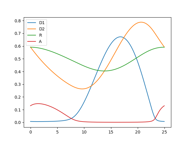
import numpy as np
from  odes.redox_oscillation import RedoxModel
from ms_package.rk_integrator import rk4
from ms_package.multiple_shooting_period import MultipleShootingPeriod
from scipy.integrate import odeint
import matplotlib.pyplot as plt
from ms_package.lma_solver_period import SolverPeriod

x = [0.5, 0.5, 0.6, 0.2]

time_array = np.linspace(0, 180, 90000)
mymodel = RedoxModel()

ms_obj =  MultipleShootingPeriod(x, M=2, period_guess= 23., t_steps=50000, model=mymodel)

mysol = SolverPeriod(ms_obj = ms_obj).lma()

jac = mysol[4]

eigenvalues, eigenvectors = np.linalg.eig(jac)


sol_array = mysol[3].space
sol_time = mysol[3].time
period = sol_time[-1]

plt.plot( sol_time, sol_array[:,0], label = "D1")
plt.plot( sol_time, sol_array[:,1], label = "D2")
plt.plot( sol_time, sol_array[:,2], label = "R")
plt.plot( sol_time, sol_array[:,3], label = "A")
plt.legend()
plt.show()

The solution is shown below:

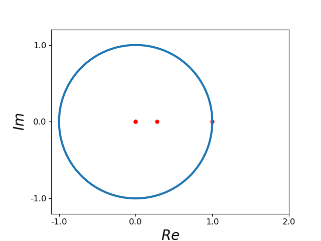
and the value of the stable Floquet multipliers is also plotted:

DOS2019

del Olmo, M.; Kramer, A.; Herzel, H, A robust model for circadian redox oscillations, Int. J. Mol. Sci. 2019, 20, 2368.