Numerical scheme

A multiple shooting algorithm is employed in order to identify the periodic orbits corresponding to trimmed flight, and to simultaneously compute their stability through their Floquet multipliers.

We use a multiple-shooting scheme first proposed by~cite{lust2001}, which was a modification of~cite{keller1968}. This algorithm is adapted to our case with the advantage that the limit cycle period is known, since it must be equal to the flapping one.

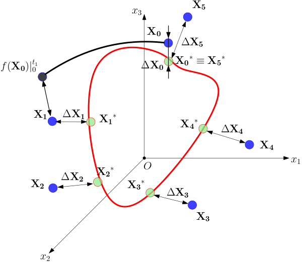
The multiple-shooting method splits the limit cycle into several points computing relatives sub-trajectories.\ Integrating the ODEs system, the point \(\mathbf{x}^*_{i+1}\) is mapped to the point \(\mathbf{x}^*_{i}\) by

(1)\[\mathbf{x}^*_{i+1} = f(\mathbf{x}^*_i) \big \rvert_{t_{i}}^{t_{i}+\tau} = f(\mathbf{x}_i + \Delta\mathbf{x}_i) \big \rvert_{t_{i}}^{t_{i}+\tau}\]

By expanding at the first order the right-hand-side of Equation (1), the point \(\mathbf{x}^*_{i+1}\) can be expressed as function of the guessed points only

(2)\[\mathbf{x}_{i+1} + \Delta\mathbf{x}_{i+1} =f(\mathbf{x}_i) \big \rvert_{t_{i}}^{t_{i}+\tau} + \mathbb{J} (\mathbf{x}_i) \Big \rvert_{t_{i}}^{t_{i}+\tau}\cdot\Delta\mathbf{x}_i\]

where \(\mathbb{J} \big \rvert_{t_{i}}^{t_{i}+\tau}(\mathbf{x}_i)\) is the Jacobian matrix previously defined.

Re-arranging Equation (2) we get

(3)\[ \mathbb{J}(\mathbf{x}_i) \Big \rvert_{t_{i}}^{t_{i}+\tau}\cdot\Delta\mathbf{x}_i -\Delta\mathbf{x}_{i+1} = \underbrace{-\big(f(\mathbf{x}_i)\big \rvert_{t_{i}}^{t_{i}+\tau} - \mathbf{x}_{i+1}\big)}_{Error}\]

and thus the multiple-shooting scheme becomes:

(4)\[\begin{split}\underbrace{ \begin{pmatrix} \mathbb{J} (\mathbf{x}_0) \Big \rvert_{0}^{\tau} & - \mathbb{I}& 0& \dots& 0 \\ \\ 0 & \mathbb{J} (\mathbf{x}_1)\Big \rvert_{t_{1}}^{t_{1}+\tau}& - \mathbb{I} & \dots & 0\\ \vdots & \vdots & \ddots & \ddots & \vdots \\ 0 & 0 &\dots & \mathbb{J}(\mathbf{x}_{m-1})\Big \rvert_{t_{m-1}}^{T} & - \mathbb{I}\\ - \mathbb{I} & 0 &\dots & 0 & \mathbb{I}\\ \end{pmatrix}}_{\mathbf{M}\ [n \times M, n \times M]} \underbrace{ \begin{pmatrix} \Delta \mathbf{x}_{0}\\ \Delta \mathbf{x}_{1}\\ \vdots\\ \vdots\\ \vdots\\ \Delta \mathbf{x}_{m-1}\\ \Delta \mathbf{x}_{m} \end{pmatrix}}_{\Delta\mathbf{x}\ [n \times M]}= \underbrace{-\begin{pmatrix} f(\mathbf{x}_0) \big \rvert_{0}^{\tau}- \mathbf{x}_1 \\ f(\mathbf{x}_1) \big \rvert_{t_{1}}^{t_{1}+\tau}- \mathbf{x}_2 \\ \vdots\\ (\mathbf{x}_{m-1}) \big \rvert_{t_{m-1}}^{T} - \mathbf{x}_m\\ \mathbf{x}_{m}- \mathbf{x}_0\\ \end{pmatrix}}_{\mathbf{E}\ [n \times M]}\end{split}\]

(5)\[\mathbf{M}(\mathbf{x}_i) \mathbf{\Delta \mathbf{x}} = \mathbf{E}(\mathbf{x}_i)\]