Stability of cycles

Given the generic system of ordinary differential equations of the form:

(1)\[\dot{\mathbf{x}} = \mathbf{v}(\mathbf{x}, t)\]

we want to find a particular solution such that:

\begin{equation} \mathbf{x}^{*}(t) = \mathbf{x}^{*}(t + T) \end{equation}

where \(T > 0\) is the period of the cycle.

Depending on their asymptotic behavior limit cycles can be either stable or unstable. In the first scenario they behave as attractors, while in the second one they behave as repellers.

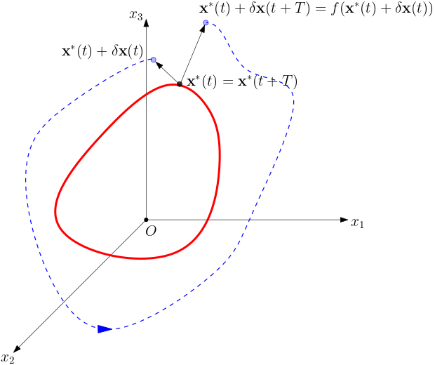
Let \(\textbf{x}^*(t) + \delta\textbf{x}(t)\) be the neighbor of a limit cycle state at time \(t\), where \(\delta\textbf{x}(t)\) thus captures the initial perturbation with respect to the limit cycle. After a time equal to the period \(T\), this point of the state space is transported by the flow as following:

(2)\[x_{i}^{*}(t) + \delta{x}_{i}(t+T) = f_{i}\big(\textbf{x}^*(t) + \delta\textbf{x}(t)\big) \Big \rvert_{t}^{t+T}\]

By expanding the right hand side of Equation (2) to the first order, and considering that \(x_{i}^{*}(t) = f_{i}\big(\textbf{x}^*(t)\big) \big \rvert_{t}^{t+T}\) (limit cycle condition), we obtain:

(3)\[\delta{x}_{i}(t+T) = \sum_{j = 1}^{N} \frac{\partial f_{i}\big(\textbf{x}^*(t)\big) \big \rvert_{t}^{t+T}}{\partial x_{j}}\cdot \delta x_j(t)\]

Equation (3) describes the dynamic of the perturbed neighboring state.

Note

The quantity

\[\mathbb{J}(\mathbf{x}^*)\big \rvert_{t}^{t+T}= \sum_{j = 1}^{N} \frac{\partial f_{i}\big(\textbf{x}^*(t)\big) \big \rvert_{t}^{t+T}}{\partial x_{j}}\]

is called the Jacobian Matrix or Floquet Matrix, and describes how the neighbor is deformed by the flow, after a period \(T\).

The stability of a periodic orbit is governed by the eigenvalues of the Jacobian matrix (Floquet multipliers). For an orbit to be stable, all the eigenvalues (except the trivial one) must be less the one in absolute value.

The Jacobian (or Monodromy) matrix, is the solution of the differential equation:

(4)\[\begin{split}\frac{d\mathbb{J}}{dt}(\mathbf{x}_0) \Big \rvert_{t_0}^{t}&= \mathbb{A}(\mathbf{x}, t) \mathbb{J}(\mathbf{x}_0) \Big \rvert_{t_0}^{t}\\ \mathbb{J} (\mathbf{x}_0)\Big \rvert_{t_0}^{t_0} &= \mathbb{I}\end{split}\]

Note

We define stability matrix the quantity

\[\mathbb{A}(\mathbf{x}, t) = \frac{\partial}{\partial x_j}v_{i(\mathbf{x}, t)}\]

where \(v\) is the right-hand-side of Equation (1)

Two methods have been implemented in the code to calculate the Jacobian matrix:

• Analytical, solving Equation (4);

• Numerical, by finite differentiation.

A multiple-shooting algorithm has been implemented in order to detect limit cycles and assess their stability.