Isothermal reaction¶

An isothermal reaction is described by a set of ODEs of the form [Sey2009]

\[\begin{split}\begin{equation} \begin{aligned} \dot{y_1} &= y_{1}(30 - 0.25y_{1} -y_{2} -y_{3}) + 0.001y_{2}^{2} + 0.1 \\ \dot{y_{2}} &= y_{2}(y_{1} - 0.001y_{2} - \lambda) + 0.1 \\ \dot{y_{3}} &= y_{3}(16.5 - y_{1} -0.5y_{3}) + 0.1 \end{aligned} \end{equation}\end{split}\]

and the relative stability matrix is therefore:

\[\begin{split}\begin{equation} \mathbb{A}(\mathbf{x}(t), t) = \begin{pmatrix} 30 - 0.5y_{1} -y_{2} -y_{3} & y_{1} + 2*0.001y_{2} & -y_{1}\\ y_{2}& y_{1} - 2*0.001y_{2} - \lambda & 0\\ -y_{3} & 0 & 16.5 - y_{1} - y_{3} \end{pmatrix} \end{equation}\end{split}\]

Generate the input file containing the ODE system and the hard code the stability matrix, inside multiflap/odes/isothermal_reaction.py:

import numpy as np

"""
Example case adopted from:

    Practical Bifurcation and Stability Analysis, page 325
    Seydel R.
    Eq. (7.15) - Isothermal chemical reaction dynamics


"""

class IsothermalReaction:
    def __init__(self, lam=1.8):
        self.lam = lam
        self.dimension=3        # specify the dimension of the problem
    def dynamics(self, x0, t):

        """ODE system
        This function will be passed to the numerical integrator

        Inputs:
            x0: initial values
            t: time

        Outputs:
            x_dot: velocity vector
        """
        y1, y2, y3 = x0
        dy1_dt = y1*(30 - 0.25*y1 -y2 -y3) + 0.001*y2**2 + 0.1
        dy2_dt = y2*(y1 - 0.001*y2 - self.lam) + 0.1
        dy3_dt = y3*(16.5 - y1 -0.5*y3) + 0.1

        vel_array = np.array([dy1_dt, dy2_dt, dy3_dt], float)
        return vel_array


    def get_stability_matrix(self, x0, t):

        """
        Stability matrix of the ODE system

        Inputs:
            x0: initial condition
        Outputs:
            A: Stability matrix evaluated at x0. (dxd) dimension
            A[i, j] = dv[i]/dx[j]
        """
        y1, y2, y3 = x0
        A_matrix = np.array([[30 - 0.5*y1 -y2 -y3, y1 + 2*0.001*y2, -y1],
                            [y2, y1 - 2*0.001*y2 -self.lam, 0.],
                            [-y3, 0., 16.5 - y1 - y3]], float)

        return A_matrix

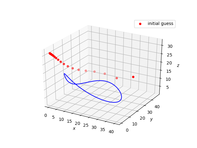
Generate the main file to run in the directory multiflap/main_isothermal.py:

import numpy as np
from  odes.isothermal_reaction import IsothermalReaction
from ms_package.multiple_shooting_period import MultipleShootingPeriod
import matplotlib.pyplot as plt
from ms_package.lma_solver_period import SolverPeriod
from mpl_toolkits.mplot3d import Axes3D

# generate the ODEs object

mymodel = IsothermalReaction(lam=11.)


# initial condition
x = [40., 20., 20.]

# generate the multiple shooting object
ms_obj = MultipleShootingPeriod(x, M=20, period_guess=.5,
                                t_steps=200, model=mymodel)

# just to plot the initial guess distribution. No need to call this
initial_guess = ms_obj.get_initial_guess()

# call the solver for the multiple-shooting algorithm
mysolution = SolverPeriod(ms_obj=ms_obj).lma()

jacobian = mysolution[4]

# Floquet multipliers
eigenvalues, eigenvectors = np.linalg.eig(jacobian)

# ODE limit cycle solution
sol_array = mysolution[3].space
sol_time = mysolution[3].time
period = sol_time[-1]

# plot the phase portrait of the limit cycle
fig1 = plt.figure(1)
ax = fig1.gca(projection='3d')
ax.set_xlabel('$x$')
ax.set_ylabel('$y$')
ax.set_zlabel('$z$')
ax.scatter(initial_guess[:,0],
           initial_guess[:,1],
           initial_guess[:,2], color='red', label='initial guess')
ax.plot(sol_array[:, 0],
        sol_array[:, 1],
        sol_array[:, 2],color = 'b')
plt.legend()
plt.show()

Run the main file inside multiflap directory:
```
python3 main_isothermal.py
```

the output will look like

Sey2009: Practical bifurcation and stability analysis, Seydel Rudiger, Springer Science & Business Media