Numerical scheme (unknown period)
What followis is a generalization of the previous scheme, suitable in all the situations where also the period of the periodic orbit is unknown.
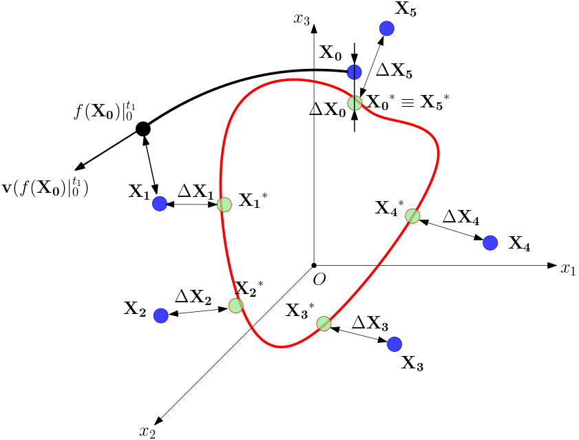
Following the same appriach as before, we split the limit cycle into several points computing relatives sub-trajectories. The relative time integration between two points, now has to be guessed as well. Mantaining the same notation, we call \(\tau^{*}\) the exact (unknown) subperiod of the periodic orbit, and \(\overline{\tau}\) the guessed subperiod of the periodic orbit. Integrating the ODEs system, the point \(\mathbf{x}^*_{i+1}\) is mapped to the point \(\mathbf{x}^*_{i}\) by
By expanding at the first order the right-hand-side of Equation (1), the point \(\mathbf{x}^*_{i+1}\) can be expressed as function of the guessed points only
Considering that
Note
We approximate the Jacobian matrix as
The function the returns the mapped point \(f(\mathbf{x}_i) \big \rvert_{t_{i}}^{t_{i}+\overline{\tau}}\) is the get_mappedpoint method of multiple_shooting_period.py module.
get_mappedpoint() Show code
def get_mappedpoint(self,x0, t0, deltat):
    """
    Returns the last element of the time integration. It outputs where a
    point x0(t) is mapped after a time deltat.

    Inputs:
        x0: initial value
        t0: initial time (required as the system is non-autonomous)
        deltat: integration_time

    Outputs:
        mapped_point: last element of the time integration
        solution: complete trajectory traced out from x0(t0) for t = deltat


    """
    t_final = t0 + deltat     # Final time

    time_array = np.linspace(t0, t_final, self.t_steps)
    if self.integrator=='rk':
        tuple_solution = rk4(self.model.dynamics, x0, time_array)
    #    sspSolution = ode.solve_ivp(birdEqn_py,
                        #[tInitial, tFinal], ssp0,'LSODA', max_step = deltat/Nt)
    #    sspSolution = (sspSolution.y).T
        solution = tuple_solution.x
        mapped_point = solution[-1, :]  # Read the final point to sspdeltat
    if self.integrator=='odeint':
        solution = odeint(self.model.dynamics, x0, time_array)
        mapped_point = solution[-1, :]
        odesol = collections.namedtuple('odesol',['x', 't'])
        tuple_solution = odesol(solution, time_array)
    return mapped_point, tuple_solution
Plugging Equation (3) in Equation (1), and re-arranging Equation (1), we get:
and thus the multiple-shooting scheme becomes:
The system (5) is set up calling the method get_ms_scheme of multiple_shooting_period.py module.
get_ms_scheme() Show code
def get_ms_scheme(self, x0, tau):


    """
    Returns the multiple-shooting scheme to set up the equation:
    MS * DX = E

    Inputs:
        x0: array of m-points of the multiple-shooting scheme

    Outputs (M = points number, N = dimension):
        MS = Multiple-Shooting matrix dim(NxM, NxM)
        error = error vector dim(NxM),
        trajectory_tuple = trajectory related to the initial value and time
    -----------------------------------------------------------------------

    Multiple-Shooting Matrix (MS):

        dim(MS) = ((NxM) x (NxM))

                 [  J(x_0, tau)  -I                                  ]
                 [              J(x_1, tau)   -I                     ]
        MS   =   [                .                                  ]
                 [                 .                                 ]
                 [                  .                                ]
                 [                        J(x_{M-1}, tau)       I    ]
                 [ -I ........................................  I    ]


    Unknown Vector:                 Error vector:

    dim(DX) = (NxM)                 dim(E) = (NxM)

            [DX_0]                          [ f(x_0, tau) - x_1 ]
    DX   =  [DX_1]                  E  =  - [ f(x_1, tau) - x_2 ]
            [... ]                          [       ...         ]
            [DX_M]                          [       x_M - x_0   ]

    """
    # The dimension of the MultiShooting matrix is (NxM,NxM)
    # The dimension of the MultiShooting matrix is (NxM,NxM)
    MS = np.zeros([self.dim*self.point_number,
                   self.dim*(self.point_number) + 1])

    # Routine to fill the rest of the scheme
    #complete_solution = []
    for i in range(0, self.point_number - 1):
        x_start = x0[i,:]
        if self.option_jacobian == 'analytical':
            jacobian = self.get_jacobian_analytical(x_start, i*tau,
                                                    tau)
        if self.option_jacobian == 'numerical':
            jacobian = self.get_jacobian_numerical(x_start, i*tau,
                                                    tau)

        MS[(i*self.dim):self.dim+(i*self.dim),
           (i*self.dim)+self.dim:2*self.dim+(i*self.dim)]=-np.eye(self.dim)


        MS[(i*self.dim):self.dim+(i*self.dim),
           (i*self.dim):(i*self.dim)+self.dim] = jacobian


        [mapped_point, complete_solution] = self.get_mappedpoint(x_start, i*tau, tau)
        last_time = complete_solution.t[-1]
        velocity = self.model.dynamics(mapped_point,last_time)
        MS[(i*self.dim):self.dim+(i*self.dim), -1] = velocity
    #trajectory = np.asanyarray(complete_solution)
    # Last block of the scheme
    MS[-self.dim:, 0:self.dim] = -np.eye(self.dim)
    MS[-self.dim:, -self.dim-1:-1] = np.eye(self.dim)
    [error, trajectory_tuple] = self.get_error_vector(x0, tau)
    print("Error vector is", error)
    return MS, error, trajectory_tuple